14. Compositional Analysis of Microbiome Data

14.1.1 What Are Compositional Data?

Composition is “the act of putting together parts or elements to form a whole” and is “the way in which such parts are combined or related: constitution” (Webster’s II New College Dictionary, 2005, p.236) [also see (Xia et al. 2018a)].  As described in Aitchison’s 1986 seminar work (Aitchison 1986b), a compositional dataset has the following four characteristics: (1) each row presents an observational unit; (2) each column presents an composition of whole; (3) each entry is non-negative; and (4) the sum of all the entries in each row equals to 1 or 100%. That is, compositional data quantitatively measure each element as a composition or describe the parts of the whole, a vector of non-zero positive values (i.e., components or parts) carrying only relative information between their components or parts (Pawlowsky-Glahn et al. 2015; Hron et al. 2010; Egozcue and Pawlowsky-Glahn 2011; Aitchison 1986a). Thus, compositional data exist as the proportions/fractions of a whole or the portions of a total (van den Boogaart and Tolosana-Delgado 2013a) and have the following unique properties: (1) The elements of the composition are non-negative and sum to unity (Bacon-Shone 2011; Xia et al. 2018a). (2) The total sum of all component values (i.e., the library size) is an artifact of the sampling procedure (Quinn et al. 2018a, b; van den Boogaart and Tolosana-Delgado 2008). (3) The difference between component values is only meaningful proportionally (Quinn et al. 2018a, b; van den Boogaart and Tolosana-Delgado 2008). The unique properties, especially adding up all the percentages of compositions necessarily to 100, introduces effects on correlations (Krumbein 1962).

14.1.2 Microbiome Data Are Treated as Compositional

Compositional data analysis is really only interested in relative frequencies rather than the absolute amount of data. Thus, compositional data analysis frequently arises in various research fields, including genomics, population genetics, demography, ecology, biology, chemistry, geology, petrology, sedimentology, geochemistry, planetology, psychology, marketing, survey analysis, economics, probability, and statistics.

14.1.3 Aitchison Simplex

Mathematically, a data is defined as compositional, if it contains D multiple parts of nonnegative numbers whose sum is 1 (Aitchison 1986a, p. 25) or any constant-sum constraint (Pawlowsky-Glahn et al. 2015, p. 10). It can be formally stated as:

(14.1)

That is, compositional data can be represented by constant sum real vectors with positive components. Where 𝜅 is arbitrary. Depending on the units of measurement or rescaling, frequent values are 1 (per unit, proportions), 100 (percent, %), (ppm, parts per million), and (ppb, parts per billion). The equation of 14.1 defines the sample space of compositional data as a hyperplane, called the simplex (Aitchison 1986a, p. 27). Also see (Mateu-Figueras et al. 2011; van den Boogaart and Tolosana-Delgado 2013a, p. 37) and (Pawlowsky-Glahn et al. 2015, p. 10). Compositional data do not exist in real Euclidean space, but rather in the simplex (a sub-space) (Aitchison 1986a).

14.1.4 Challenges of Analyzing Compositional Data

Standard methods (e.g., correlation analysis) rely on the assumption of Euclidean geometry in real space (i.e., P) (Eaton 1983) and assume that the differences between the tested variables are linear or additive. However, the simplex has one dimension less than real space (i.e., P-1), which represent special properties of the sample space (Aitchison 1986a). Therefore, in compositional data each component (or part) of the whole is dependent on other components. Because the sum of all proportions of each component equals to 1 (100%), at least two components are negatively correlated. This results in the dependency problem of the measured variables (e.g., taxa/OTUs/ASVs). In the statistical and especially in current microbiome literatures, the issue of dealing with proportions is referred as to compositionality. Microbial abundances are typically interpreted as proportions (e.g., relative abundance) to account for differences in sequencing depth (see Sect. 14.1.2 for details). Because proportions add to one, the change of a single microbial taxon will also change the proportions of the remaining microbial taxa. Therefore, it poses a challenge to infer exactly which microbial taxon is changing with treatments or conditions.

14.1.5 Fundamental Principles of Compositional Data Analysis

Aitchison proposed and suggested (Aitchison 1982, 1986a) three fundamental principles for the analysis of compositional data that we should adhere to when analyzing compositional data. These fundamental principles are all rooted in the definition of compositional data: only ratios of components carry information and have been reformulated several times according to new theoretical developments (Barceló-Vidal et al. 2001; Martín-Fernández et al. 2003; Aitchison and Egozcue 2005; Egozcue 2009; Egozcue and Pawlowsky-Glahn 2011). The three fundamental principles are: (1) scaling invariance; (2) subcompositional coherence; and (3) permutation invariance.

In 2008, Aitchison summarized basic principle of compositional data analysis. For its formal expression, we cannot do better than to quote his definition (Aitchison 2008):

Other important properties of CoDa include perturbation invariance and subcompositional dominance. Perturbation invariance states that converting a composition between equivalent units will not change the results (van den Boogaart and Tolosana-Delgado 2013b; Quinn et al. 2018a, b).

Subcompositional dominance states that using a subset of a complete composition carries less information than using the whole (van den Boogaart and Tolosana-Delgado 2013b; Quinn et al. 2018a, b).

14.1.6 The Family of Log-Ratio Transformations

Compositional data exist in the Aitchison simplex (Aitchison 1986a), while the most statistical methods or models are valid in Euclidean space (real space). Aitchison (1981, 1982, 1983, 1984, 1986a; Aitchison and Egozcue 2005) approved that compositional data could be mapped into Euclidean space by using the log-ratio transformation and then can be analyzed using standard statistical methods or models such as an Euclidean distance metric (Aitchison et al. 2000). Thus, usually most compositional data analyses start with a log-ratio transformation (Xia et al. 2018a).

The algorithm behind the log-ratio transformation principle is that compositional vectors and associated log-ratio vectors exist a one-to-one correspondence so that any statement about compositions can be reformed in terms of log-ratios and vice versa (Pawlowsky-Glahn et al. 2015). Thus, log-ratio transformations solve the problem of a constrained sample space by projecting compositional data in the simplex into multivariate real space. Therefore, open up all available standard multivariate techniques (Pawlowsky-Glahn et al. 2015).

In order to transform the simplex to the real space, Aitchison in his seminal work (1986a, b) developed a set of fundamental principles, a variety of methods, operations, and tools, including the additive log-ratio (alr) for compositional data analysis.

The log-ratio transformation methodology has been accepted in various fields such as geology and ecology (Pawlowsky-Glahn and Buccianti 2011; van den Boogaart and Tolosana-Delgado 2013a; Aitchison 1982; Pawlowsky-Glahn et al. 2015). Here, we introduce the family of log-ratio transformations including the additive log-ratio (alr) (Aitchison 1986a, p. 135), the centered log-ratio (clr) (Aitchison 2003), the inter-quartile log-ratio (iqlr) (Fernandes et al. 2013, 2014), and isometric log-ratio (ilr) (Egozcue et al. 2003) transformations.

14.1.6.1 Additive Log-Ratio (alr) Transformation

The original approach of compositional data analysis proposed in Aitchison (1986a, b) was based on the alr-transformation. It is defined as:

(14.2)

This formula maps a composition in the D-part Aitchison simplex none isometrically to a D-1 dimensional Euclidean vector. The alr-transformation chooses one component as a reference and takes the logarithm of each measurement within a composition vector (i.e., in the microbiome case, each sample vector containing relative abundances) after divided by a reference taxon (usually the taxon with index D, with D being the total number of taxon is chosen). Sum of all X_j to unity, but we can replace the components with any observed counts, which do not change the expression due to the library sizes cancelation. After the alr-transformation, any separation between the groups revealed by the ratios can be analyzed by standard statistical tools (Thomas and Aitchison 2006).

14.1.6.2 Centered Log-Ratio (clr) Transformation

The clr-transformation is defined as the logarithm of the components after dividing by the geometric mean of x:

(14.3)

with ensuring that the sum of the elements of clr(x) is zero. Where x = (x₁, …, x_i, …, x_D) represents the composition. The clr-transformation maps a composition in the D-part Aitchison simplex isometrically to a D-1 dimensional Euclidean vector. Unlike the alr-transformation in which a specific taxon is used as reference, the clr-transformation uses the geometric mean of the composition (i.e., sample vector) in place of x_D. Like the alr, after performing the clr-transformation, the standard unconstrained statistical methods can be used for analyzing compositional data (Aitchison 2003).

The clr-transformation algorithm has been adopted by some software (van den Boogaart and Tolosana-Delgado 2013b; Fernandes et al. 2013), and it was shown it could be used to analyze microbiome data and RNA-seq data and other next-generation sequencing data (Fernandes et al. 2014).

14.1.6.3 Isometric Log-Ratio (ilr) Transformation

The ilr-transformation is defined as:

(14.4)

where,

Like the clr, the ilr-transformation maps a composition in the D-part Aitchison simplex isometrically to a D-1 dimensional Euclidian vector. This ilr-transformation is an orthonormal isometry. It is the product of the clr and the transpose of a matrix which consists of elements. The elements are clr-transformed components of an orthonormal basis. The ilr-transformation transforms the data regarding an orthonormal coordinate system that performed from sequential binary partitions of taxa (van den Boogaart and Tolosana-Delgado 2013b).

Like alr and clr, ilr-transformation was developed to transform compositional data from the simplex into real space where standard statistical tools can be applied (Egozcue and Pawlowsky-Glahn 2005; Egozcue et al. 2003). That is, the ilr-transformed data can be analyzed using the standard statistical methods.

14.1.7 Remarks on Log-Ratio Transformations

Due to these limitations and specifically the difficulty to interpret the results. In practice, ilr has somewhat limited its adoption or application (Egozcue et al. 2003; Xia et al. 2018a).

Compared to other three log-ratio transformations, the iqlr-transformation is not getting widely applied.

14.2.1 Introduction to ALDEx2

ALDEx (Fernandes et al. 2013) and ALDEx2 (Fernandes et al. 2014) were initially developed for analyzing differential expression of mixed population RNA sequencing (RNA-seq) data, but it has been showed that this approach is essentially generalizable to nearly any type of high-throughput sequencing data, including three completely different experimental designs: the traditional RNA-seq, 16S rRNA gene amplicon-sequencing, and selective growth-type (SELEX) experiments (Fernandes et al. 2014; Gloor and Reid 2016; Gloor et al. 2016; Urbaniak et al. 2016). The R packages called ALDEx and ALDEx2 have been used to analyze unified high-throughput sequencing datasets such as RNA-seq, chromatin immunoprecipitation sequencing (ChIP-seq), 16S rRNA gene sequencing fragments, metagenomic sequencing, and selective growth experiments (Fernandes et al. 2014).

High-throughput sequencing (e.g., microbiome) data have several sources of variance including sampling replication, technical replication, variability within biological conditions, and variability between biological conditions. ALDEx and ALDEx2 were developed in a traditional ANOVA-like framework that decompose sample-to-sample variation into four parts: (1) within-condition variation, (2) between-condition variation, (3) sampling variation, and (4) general (unexplained) error.

Fernandes et al. (2013) highlighted the importance for partitioning and comparing biological between-condition and within-condition differences (variation), and hence they developed ALDEx, an ANOVA-like differential expression procedure, to identify genes (in the case, taxa/OTUs) with greater between- to within-condition differences via the parametric Welch’s t-test or a non-parametric testing such as Wilcoxon rank sum test or Kruskal-Wallis test (Fernandes et al. 2013, 2014).

ALDEx was developed using the equivalency between Poisson and multinomial processes to infer proportions from counts and model the data as “compositional” or “proportional.” In other words, ALDEx2 uses log-ratio transformation rather than effective library size normalization in count-based differential expression studies. However, when sample sizes are small, the marginal proportions have the large variance and extremely not normally distributed. Thus, ALDEx performs all inferences based on the compositionally valid Dirichlet distribution, i.e., using the full posterior distribution of probabilities drawn from the Dirichlet distribution through Bayesian techniques.

Like other CoDa approaches, ALDEx is not interested in the total number of reads, instead of inferring proportions from counts. Denote n_i present the number of counts observed in taxon i, and assume that each taxon’s read count was sampled from a Poisson process with rate μ_i, i.e., n_i~Poisson(μ_i) with n = ∑_in_i. Then, the set of joint counts with given total read counts has a multinomial distribution, i.e., {[n₁, n₂, …]| n} ~ Multinomial (p₁, p₂, …| n) where each p_i = μ_i/∑_kμ_k based on the equivalency between Poisson and multinomial processes.

Since the Poisson process is equivalent to the multinomial process, traditional methods use n_i to estimate μ_i and then use the set of μ_i to estimate p_i. These methods ignore that most datasets of this type contain large numbers of taxa with zero or small read counts; thus the maximum-likelihood estimate of p_i this way is often exponentially inaccurate. Therefore, ALDEx estimate the set of proportions p_i directly from the set of counts n_i. ALDEx uses standard Bayesian techniques to infer the posterior distribution of [p₁, p₂, …] as the product of the multinomial likelihood with a Dirichlet (, ,…) prior. Considering the large variance and extreme non-normality of the marginal distributions p_i when the associated n_i are small, ALDEx does not summarize the posterior of p_i using point-estimates. Instead, it performs all inferences using the full posterior distribution of probabilities drawn from the Dirichlet distribution such that [p_i, p₂, …]~ Dirichlet . Adding 0.5 to the Dirichlet distribution, the multivariate distribution avoids the zero problem for the inferred proportions even if the associated count is zero and conserves the probability, i.e., ∑_kp_k = 1.

Because mathematically log-proportions are easily manipulated, ALDEx takes the component-wise logarithms and subtracts the constant from each log-proportion component for a set of m proportions [p_i, p₂, …, p_m]. This results in the values of the relative abundances where ∑_kq_k is always zero. Most important, it projects q onto a m − 1 dimensional Euclidean vector space with linearly independent components. Thus, a traditional ANOVA-like framework can be formed to analyze the q values [q_i, q₂, …, q_m].

Because it is cumbersome to directly compute q distribution, the software estimates the distribution of q from multiple Monte Carlo realizations of p given [n₁, n₂, …n_m]. MC sampling is based on the compositionally valid Dirichlet distribution with the addition of a uniform prior. That is, it repeats the MC sampling for K times (K = 128 times by default) and consequently creating randomized instances dataset, in which for each taxon i in sample j, the observed abundance O_ij is represented by a vector of MC samples of relative abundances . This renders the data free of zeros.

• Part 2: Perform log-ratio transformation on each of the so-called Monte Carlo (MC) instances usually most through clr- or iqlr-transformation

After obtaining the multivariate Dirichlet proportional distributions, to make a meaningful comparison between-sample values from proportional distributions, ALDEx uses the procedures developed by Aitchison, Egozcue, and others (Aitchison and Egozcue 2005; Egozcue and Pawlowsky-Glahn 2005; Egozcue et al. 2003) to transform component proportions into linearly independent components. That is, it performs the relative abundance vector for each sample j and each MC Dirichlet realization k, k = 1, …, K. The distributions are estimated from multiple independent Monte Carlo realizations of their underlying Dirichlet-distributed proportions for all taxa (genes) i simultaneously.

• Part 3: Perform statistical hypothesis testing on each MC instance, i.e., each taxon in the vector of clr or iqlr transformed values, to generate P-values (P) for each transcript

The hypothesis testing is performed using the classical statistical tests, i.e., Welch’s t and Wilcoxon rank sum tests for two groups, and glm and Kruskal-Wallis for two or more groups. Since there is a total of K MC Dirichlet samples, each taxon will have K P-values.

Let i = {1, 2, …, I} index taxa (genes), j = {1, 2, …, J} index the groups (conditions), and k = {1, 2, …, K_j} index the replicate of a given group(condition), using the framework of random-effect ANOVA models, the ALDEx model is given as below.

(14.5)

where q_ijk is the adjusted log-abundance (expression); μ_ij is the expected abundance (expression) of taxon i (gene i) within each group (condition) j; ν_ijk is the sample-specific abundance (expression) change for replicate k; τ_ijk is the sampling variation from inferring abundance (expression) from read counts; and ε_ijk is the remaining nonspecific error.

Here, ν_ijk is assumed to be approximately normal as in the usual ANOVA models. The sampling error τ_ijk is given by the adjusted log-marginal distributions of the Dirichlet posterior and its distribution is very Gaussian-like. To ensure it is more appropriate for the analysis of high-throughput sequencing datasets, ALDEx does not assume that within-group (condition) sample-to-sample variation is small and essentially negligible.

Under the ANOVA framework, ALDEx conducts a null hypothesis to test the difference between groups (conditions) j and j^′, for all taxa i (genes i).

• Part 4: Average these P-values across all MC instances to yield expected P-values for each taxon.

The expected P-values are Benjamini-Hochberg adjusted P-values (BH) by using Benjamini-Hochberg correction procedure (Benjamini and Hochberg 1995).

The authors of this model (Fernandes et al. 2013) emphasize the statistical significance by this hypothesis testing in Part 3 above does not imply that the groups (conditions) j and j^′ are meaningfully different. Instead, such meaning can be inferred through an estimated effect size that compares predicted between group (condition) differences to within-group(condition) differences.

Given the set of random variables p_ijk and q_ijk, the within-group (condition) distribution is:

(14.6)

the absolute fold difference between-group (condition) distribution is:

(14.7)

the between sample, within-group(condition) difference is:

(14.8)

and the relative effect size:

(14.9)

The effect size metric in ALDEx2 is another statistical method that was developed specifically for this package and is recommended for use over the P-values.

For normally distributed data, usually effect sizes measure the standardized mean difference between groups, such as Cohen’s d (1988) measures the standardized difference between two means. Cohen’s d has been widely used in behavioral sciences accompanying reporting of t-test and ANOVA results and meta-analysis. However, in high-throughput sequencing data, the data are often not normally distributed. For non-normality of data, it is very difficult to measure effect sizes and interpret them.

ALDEx2 effect size measure estimates the median standardized difference between groups. It is a standardized distributional effect size metric. To obtain this effect size, take the median of differences (about -2), which provides a non-parametric measure of the between-group difference. Then, scale (normalize) the median of differences by the dispersion: effect = median (difference / dispersion). Where dispersion = maximum (vector a-randomly permutated vector a, vector b- randomly permutated vector b). In the aldex.effect module output, these measures are denoted as: diff.btw = median(diff), diff.win = median(disp), and effect = eff. ALDEx2 also provides a 95% confidence interval of the effect size estimate if in the aldex.effect() function, CI=TRUE is specified (see Sect. 14.2.2).

It was shown that ALDEx2 effect size is somewhat robust and is approximately 1.4 times that of Cohen’s d, as expected for a well-behaved non-parametric estimator. It is equally valid for normal, random uniform, and Cauchy distributions (Fernandes et al. 2018).

14.2.2 Implement ALDEx2 Using R

ALDEx2 takes the compositional data analysis approach that uses Bayesian methods to infer technical and statistical error (Fernandes et al. 2014). ALDEx2 incorporates a Bayesian estimate of the posterior probability of taxon abundance into a compositional framework; that is, it uses a Dirichlet distribution to transform the observed data and then estimates the distribution of taxon abundance by random sampling instances of the transformed data. There are two essential procedures: ALDEx2 first takes the original input data and generates a distribution of posterior probabilities of observing each taxon; then it uses the centered log-ratio transformation to transform this distribution. After centered log-ratio transforming the distribution, a parametric or nonparametric t-test or ANOVA can be performed for the univariate statistical tests and the P-values and Benjamini-Hochberg adjusted P-values are returned.

The ALDEx2 methods are available from the ALDEx2 package (current version 1.27.0, October 2021). There are three approaches that can be used to implement ALDEx2 methods: (1) Bioconductor ALDEx2 modular, (2) ALDEx2 wrapper, and (3) the aldex.glm module. Bioconductor version of ALDEx2 is modular, which is achieved by exposing the underlying center log-ratio transformed Dirichlet Monte-Carlo replicate values and hence is flexible for adding the specific R commands by the users based on their experimental design. Thus, it is suitable for the comparison of many different experimental designs. Currently, the ALDEx2 wrapper is limited to a two-sample t-test (and calculation of effect sizes) and one-way ANOVA design. The aldex.glm module was developed to implement the probabilistic compositional approach for complex study designs.

We illustrated this package in our previous book (Xia et al. 2018a). In this section, we illustrate these three approaches in turn with a new microbiome dataset.

The aldex.ttest() returns the values of we.ep (expected P-value of Welch’s t test), we.eBH (expected Benjamini-Hochberg corrected P-value of Welch’s t test), wi.ep (expected P-value of Wilcoxon rank test), and wi.eBH (expected Benjamini-Hochberg corrected P-value of Wilcoxon test).

As an alternative method of the t-test, we can run the aldex.kw module to perform the Kruskal-Wallis and glm tests for one-way ANOVA, which compares two or more groups.

The following head () function examines the first three lines of data.

> head(aldex_all,3)

we.ep we.eBH wi.ep wi.eBH rab.all rab.win.KO rab.win.WT

OTU_2 0.5406304 0.8283945 0.5739729 0.8502291 -1.328501 -1.536681 -1.1439323

OTU_3 0.4959608 0.8083920 0.5036120 0.8216989 -1.150645 -1.359854 -0.8576377

OTU_4 0.4926840 0.7968770 0.5281530 0.8168477 -1.243212 -1.427288 -1.0419705

diff.btw diff.win effect effect.low effect.high overlap

OTU_2 0.4165297 4.331159 0.08838384 -3.629842 4.652759 0.4515625

OTU_3 0.3566450 4.210935 0.07741749 -3.017144 5.117261 0.4531250

OTU_4 0.3932742 4.087157 0.07952276 -3.702736 4.159538 0.4578125

• Step 6: Run the aldex.plot module to generate the MA and MW (effect) plots.

• Bland-Altman plot (difference plot, or Tukey mean-difference plot), named after J. Martin Bland and Douglas G. Altman, is a data plotting method for analyzing the agreement between two different measures (Altman and Bland 1983; Martin Bland and Altman 1986; Bland and Altman 1999). Bland-Altman method states that any two methods designing to measure the same property or parameter are not merely highly correlated but also should have agreed sufficiently closely. ALDEx2 provides a Bland-Altman (MA) style plot to graphically compare the degree of agreement of measures between median log₂ between-condition difference and median log₂ relative abundance.

• Effect size in ALDEx2 is defined as a measure of the mean ratio of the difference between groups (diff.btw) and the maximum difference within groups (diff.win or variance). The effect size can be obtained by the aldex.effect modular or by specifying effect=TRUE argument using the aldex wrapper. The aldex.plot modular plots median between-group difference versus median within-group difference to visualize differential abundance of the sample data, which are referred to as “effect size” plots in ALDEx2.

• The following commands generate the MA and MW (effect) plots (Fig. 14.1).

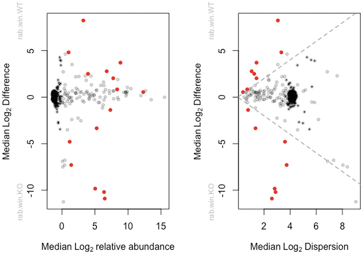
Two scatterplots of median log subscript 2 difference versus median log subscript 2 relative abundance and median log subscript 2 dispersion plot dots in red, gray, and black colors.

ALDEx2 generates a posterior distribution of the probability of observing the count given the data collected. Importantly this approach generates the 95% CI of the effect size. ALDEx2 uses a standardized effect size, similar to the Cohen’s d metric. It was shown the effect size in ALDEx2 is more robust and more conservative (being approximately 0.7 Cohen’s d when the data are normally distributed based on Greg Gloor’s note in his AlDEx2_vignette of ANOVA-Like Differential Expression tool for high throughput sequencing data, October 27, 2021).

In general, P-value is less robust than effect size. Thus, more researchers prefer to report effect size than to P-value. If sample size is sufficiently large, an effect size of 0.5 or greater is considered more likely corresponding to biological relevance.

A few features have an expected Q-value that is statistically significantly different. They are both relatively rare and have a relatively small difference. For those features, it can be misleading even when identifying them based on the expected effect size. ALDEx2 finds that the safest approach to identify those features is to find where the 95% CI of the effect size does not cross 0. The 95% CI metric behaves exactly in line with intuition: the precision of estimation of rare features is poor. To identify rare features with more confidence, more deep sequencing is required. The authors of ALDEx2 think this 95% CI approach can identify the biological variation in the data as received (i.e., the experimental design is always as given). This is the approach that was used in Macklaim et al. (2013), and it was independently validated to be very robust (Nelson et al. 2015). In summary, this approach is not inferring any additional biological variation but is identifying those features where simple random sampling of the library would be expected to give the same result every time.

ALDEx2 considers an effect size cutoff of 1.5–2 and an overlap cutoff of 0.01 as more appropriate to identify differential taxa of interest (Fernandes et al. 2013). Below we illustrate two more effect size plots: (1) plot the effect size versus the P-value, and (2) a volcano plot shows the difference between groups versus the P-value (Fig. 14.2).

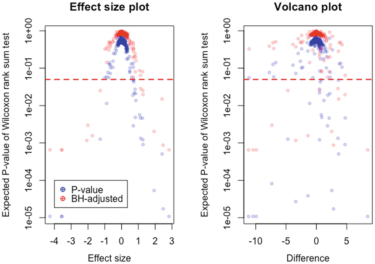
2 graphs. An effect size plot of expected P value of Wilcoxon rank sum test versus effect size and a volcano plot of expected P value of Wilcoxon rank sum test versus difference. A dotted line is between 1 e 01 and 1 e 02. Dots for P and B H adjusted values are crowded above the line.

Twenty seven taxa are identified as significant by both Welch’s t-test and Wilcoxon rank sum test, and twelve of these reach significance when the P-values are adjusted for multiple testing corrections using the Benjamini-Hochberg’s method.

The following R commands use the xtable() function from xtable package to make a result table. The xtable package is used to create export tables, converting an R object to an xtable object, which can then be printed as a LaTeX or HTML table. Here, the print.xtable() function is used to export to HTML file. If you want to export the LaTeX file, then use type="latex", file="ALDEx2_Table_Coef_QtRNA.tex" instead.

Only those significant taxa detected in both Welch’s t-test and Wilcoxon rank sum tests are printed in Table 14.1. We can interpret the table this way, for the OTU_98, the absolute difference between KO and WT groups can be up to −4.698, implying that the absolute fold change in the ratio between OTU_98 and all other taxa between KO and WT groups for this organism is on average (1/2)^−4.698 = 25.96 fold across samples. The difference within the groups of 3.539 is roughly equivalent to the standard deviation, giving an effect size of −4.698/3.539 = −1.327 (here exactly: −1.269 [−9.010, 0.347]).

Here the test group ‘Genotype’ has two levels (KO vs. WT). So this is two-sample t-test. We specify test = “t,” and then the effect should be set to TRUE. The “t” option evaluates the data as a two-factor experiment using both Welch’s t-test and the Wilcoxon rank sum test. Like other tests, t-tests also include a Benjamini-Hochberg correction of the raw P-values. The data also can be plotted onto Bland-Altman (MA) or effect (MW) plots (Fig. 14.3).

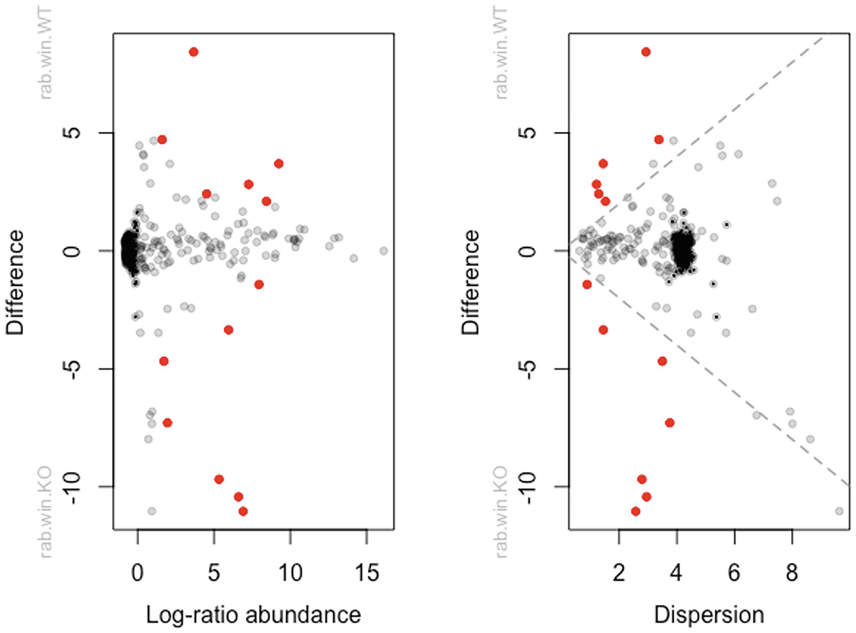
Two scatterplots of difference versus log-ratio abundance and dispersion plots dots in red, gray, and black colors.

The inter-quartile log-ratio (iqlr) transformation was introduced in the ALDEx2 package (see Sect. 14.1.6.4). The following commands use iqlr transformation and generate MA and MW plots.

The left panel is an Bland-Altman (MA) plot that shows the relationship between (relative) abundance and difference. The right panel is an MW (effect) plot that shows the relationship between difference and dispersion. In both plots, red dots indicate that the features are statistically significant and gray or black dots indicate the features are not significant. The log-ratio abundance axis is the clr value for the feature.

Figure 14.4 can be generated using the following R commands, which plots the BH-corrected glm values for the actual test case vs. the effect size for the binary predictor.

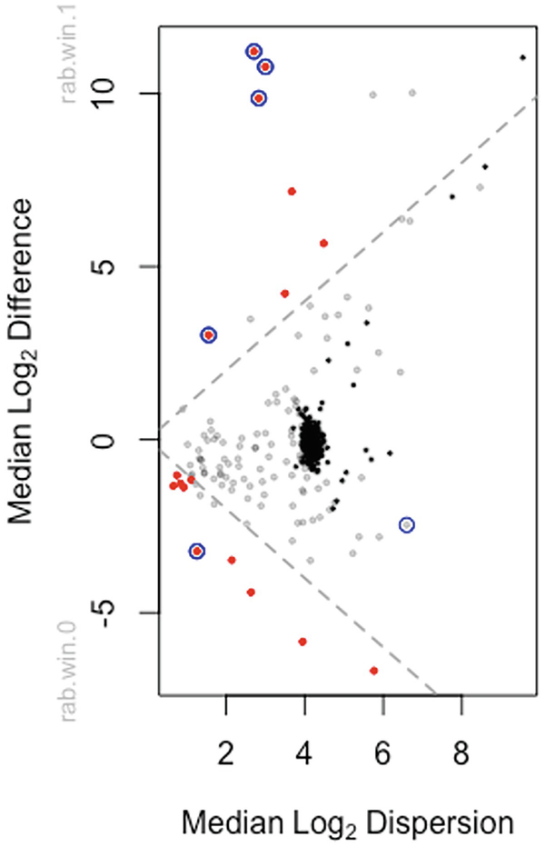
A scatterplot of median log subscript 2 difference versus median log subscript 2 dispersion plots dots in red, gray, and black colors. 2 dotted lines from (0, 0) increase and decrease, respectively.

14.2.3 Remarks on ALDEx2

ALDEx2 was reported having difficulty to control FDR (Lin and Peddada 2020b) and to maintain statistical power compared to competing differential abundance methods (e.g., ANCOM, ANCOM-BC, edgeR, and DESeq2) (Lin and Peddada 2020b; Morton et al. 2019).

14.3.1 Introduction to ANCOM

ANCOM (Mandal et al. 2015), an alr (additive log-ratio)-based method, was proposed based on alr-transformation to account for the compositional structure of microbiome data. ANCOM repeatedly uses alr-transformation to choose each of the taxa in the dataset as a reference taxon at a time. Thus, given a total of m taxa, ANCOM will choose each of the m taxa to be a reference taxon one time and repeatedly perform the alr-transformation for each taxon and m − 1 regressions. Therefore, total m(m − 1) regression models will be fitted.

Like an ANOVA model, ANCOM models the log-ratios of OTU abundances in each sample with a linear model, but, unlike typical ANOVA, ANCOM accommodates dependencies and correlations among the relative abundances of the OTUs by using of log-ratios. That is, ANCOM lies on framework of ANOVA, while accounts for the compositional structure of microbiome data. The dependencies and hence compositional structure arise in microbiome data because the relative abundances of OTUs sum to 1 or 100% in each sample and because relative abundances of different OTUs may be positively or negatively correlated.

Under these two assumptions, for the i^th taxon and j^th sample, ANCOM developed a statistical model using a standard ANOVA model formulation to perform all possible DA analyses by successively using each taxon as a reference taxon.

(14.10)

where i^′ is the reference taxon, i^′ ≠ i = 1, 2, …, m, and g = 1, 2, …, G is the number of study groups.

• Part 2: Conduct a null hypothesis regarding mean log absolute abundance in a unit volume of an ecosystem using relative abundances.

It was shown (Mandal et al. 2015) that by combining these two assumptions, it can conduct a null hypothesis regarding mean log absolute abundance in a unit volume of an ecosystem using relative abundances. And to test whether a taxon i is differentially abundant regarding a factor of interest with G levels is equivalent to test the null hypothesis and the alternative hypothesis (Lin and Peddada 2020b):

• Part 3: Adjust the P-values from the tests of taxon.

There are P-values from the tests of taxon. ANCOM uses Benjamini-Hochberg (BH) procedure (Benjamini and Hochberg 1995) or Bonferroni correction procedure (Dunn 1958, 1961) to adjust the P-values for a multiple testing correction. For each taxon, the number of rejections W_i is based on the empirical distribution of {W₁, W₂, …, W_m}, which determines the cutoff value of significant taxon (Mandal et al. 2015). The large value of W_i indicates that taxon i is more likely differentially abundant. However, the decision rule of choosing cutoff value of W_i is kind of arbitrary in ANCOM, although 70th percentile of the W distribution is recommended. The users can select different threshold of cutoff value such as the 60th to 90th to output the statistical testing results.

14.3.2 Implement ANCOM Using QIIME 2

ANCOM assumes that less than about 25% of the features are changing between groups. If this assumption is violated, then ANCOM will be more possible to increase both Type I and Type II errors. As we showed in Chap. 10 via emperor plot that a lot of features were changed in abundance over time (Early and Late times), here we will filter the full feature table to only contain late mouse gut samples and then perform ANCOM to identify which sequence variants and taxa are differentially abundant across the male and female mouse gut samples.

A text reads, saved feature table, open bracket, frequency, close bracket, to, L a t e M o u s e G u t T a b l e dot q z a.

A text reads, saved feature table, open bracket, frequency, close bracket, to, L a t e M o u s e G u t T a b l e 2 dot q z a.

A text reads, saved feature table, open bracket, frequency, close bracket, to, L a t e M o u s e G u t T a b l e 3 dot q z a.

A text reads, saved feature table, open bracket, frequency, close bracket, to, L a t e M o u s e G u t T a b l e L 6 dot q z a.

A text reads, saved feature table, open bracket, frequency, close bracket, to, L a t e M o u s e G u t T a b l e L 7 dot q z a.

The following intermediate files can be removed from the directory by rm command, such as rm LateMouseGutTable.qza. However, we keep them there for later review.

As a compositional method, ANCOM cannot address zero issue because frequencies of zero are not defined when taking log or log-ratio transformation. ANCOM operates on a FeatureTable[Composition] QIIME 2 artifact, which is based on frequencies of features on a per-sample basis. To build the composition artifact (a FeatureTable[Composition] artifact), a small pseudocount must be added to the FeatureTable[Frequency] artifact typically via an imputation method.

A text reads, saved feature table, open bracket, composition, close bracket, to, C o m p L a t e M o u s e G u t T a b l e L 6 dot q z a.

A text reads, saved feature table, open bracket, composition, close parenthesis, to, C o m p L a t e M o u s e G u t T a b l e L 7 dot q z a.

A text reads, saved visualization to, A n c o m S e x M i s S e q underscore S O P L 6 dot q z v.

A text reads, saved visualization to, A n c o m S e x M i s S e q underscore S O P L 7 dot q z v.

This view command displays three results: (1) ANCOM Volcano Plot, (2) ANCOM statistical results, and (3) percentile abundances of features by group. All these results can be exported, downloaded, and saved.

A text reads, saved feature table open bracket, composition, close bracket, to, c o m p L a t e M o u s e G u t T a b l e dot q z a.

A text reads, saved visualization to, A n c o m S e x M i s S e q underscore S O P dot q z v.

ANCOM provides two optional parameters --p-transform-function and --p-difference-function to perform identity differential features. Both parameters are TEXT choices [(‘sqrt’, ‘log’, ‘clr’), (‘mean_difference’, ‘f_statistic’) for --p-transform-function and --p-difference-function, respectively]. The transform-function is used to specify the method to transform feature values before generating volcano plots. The default is “clr” (centered log ratio-transformation). Other two are square root (“sqrt”) and log (“log”) transformations. The difference-function is used to specify the method to visualize fold difference in feature abundances across groups for volcano plots. One command is provided below.

A text reads, saved visualization to, A n c o m S e x M i s S e q underscore S O P L 7 dot q z v.

14.3.3 Remarks on ANCOM

14.4.1 Introduction to ANCOM-BC

ANCOM-BC (Lin and Peddada 2020a) was proposed for differential abundance (DA) analysis of microbiome data with bias correction to ANCOM. ANCOM-BC was developed under the assumptions that (1) the observed abundance in a feature table is expected to be proportional to the unobservable absolute abundance of a taxon in a unit volume of the ecosystem. (2) The sampling fraction varies from sample to sample and hence inducing the estimation bias. Thus, to address the problem of unequal sampling fractions, ANCOM-BC uses a sample-specific offset term to serve as the bias correction (Lin and Peddada 2020a). The offset term is usually used in the generalized linear models such as Poisson, zero-inflated models to adjust for the sampling population (Xia et al. 2018b). Here ANCOM-BC uses a sample-specific offset term in a linear regression framework.

Unlike some other DA studies, which defines relative abundances of taxa as frequencies of these taxa in a sample, in ANCOM-BC, relative abundance of a taxon in the sample refers to the fraction of the taxon observed in the feature table relative to the sum of all observed taxa corresponding to the sample in the feature table (Lin and Peddada 2020a, b). Actually, it is the proportion of this taxon relative to the sum of all taxa in the sample with range of (0, 1). In ANCOM-BC, absolute abundance is defined as unobservable actual abundance of a taxon in a unit volume of an ecosystem, while observed abundance refers to the observed counts of features (OTUs or ASVs) in the feature table (Lin and Peddada 2020b).

Let O_ij denote the observed abundance of i^th taxon in j^th sample, A_ij the unobserved abundance of i^th taxon in the ecosystem of i^th sample, and then the sample-specific sampling fraction c_j is defined as:

(14.11)

where c_j is the ratio of the expected abundance of taxon i in the j^th sample to its absolute abundance in a unit volume of an ecosystem such as gut where the sample was derived from, which could be empirically estimated by the ratio of library size to the microbial load.

Assumption 1 is given below.

(14.12)

where is the variability between specimens within the k^th sample from the j^th group, which characterizes the within-sample variability. Usually the within-sample variability is not estimated since typically at a given time only one specimen is available in most microbiome studies. The assumption in (14.12) states that the absolute abundance of a taxon in a random sample is expected to be in constant proportion to the absolute abundance in the ecosystem of the sample. That is, the expected relative abundance of each taxon in a random sample equals to the relative abundance of the taxon in the ecosystem of the sample (Lin and Peddada 2020a).

Assumption 2 is given below. For each taxon i, A_ijk, j = 1, …, g, k = 1, …, n_j, are independently distributed with

(14.13)

where θ_ij is a fixed parameter rather than a random variable; is the between-sample variation within group j for the i^th taxon. The assumption in (14.13) states that for a given taxon, all subjects within and between groups are independent.

Combining Assumption 1 in (14.12) and Assumption 2 in (14.13), the expected and variance of O_ijk are defined as:

(14.14)

• Part 3: Introduce a linear regression model framework for log-transformed OTU counts data to include the sample specific bias due to sampling fractions.

Under the above setting, the linear model framework for log-transformed OTU counts data is written as below.

(14.15)

where

(14.16)

Since the sample-specific bias is introduced because of the differential sampling fraction by each sample, thus, the goal of ANCOM-BC is to eliminate this bias. Given a large number of taxa on each subject, to estimate this bias, ANCOM-BC borrows information across taxa in its methodology.

The framework of least squares was used to develop bias and variance of bias estimation under the null hypothesis, which are estimated as follows.

(14.17)

where note that . Thus, for each j = 1, 2, …, g, Lin and Peddada (2020a) approve that is a biased estimator and For two experimental groups with balanced design (i.e., g = 2 and n₁ = n₂ = n) and given two ecosystems, for each taxon i, i = 1, ⋯, m, the test hypotheses are

By denoting , under the null hypothesis, and hence is biased. From (12.15) and Lyapunov central limit theorem, Lin and Peddada (2020a) show that

(14.18)

where Lin and Peddada (2020a) show that the taxa can be modeled using a Gaussian mixtures model and the expectation-maximization (EM) algorithm (i.e., , which denotes the resulting estimator of δ). They also show that that and (denoting the weighted least squares (WLS) estimator of δ) are highly correlated, are approximately unbiased, and thus can use to approximate for .

Therefore, under some further assumptions and developments, for hypothesis testing for two-group comparison: for taxon i , the following test statistic is approximately centered at zero under the null hypothesis:

(14.19)

From Slutsky’s theorem,

(14.20)

The above test statistic is modified as follows if the sample size is not very large and/or the number of non-null taxa is very large:

(14.21)

• Part 5: Adjust the P-values from the tests of taxon.

The test statistic for multigroup comparison was developed in the same way to the two-group comparison. That is, first getting the initial estimates of and , then setting the reference group r (e.g., r = 1), and obtaining the estimator of the bias term through E-M algorithm, the final estimator of mean absolute abundance of the ecosystem (in log scale) are obtained by transforming of (14.17) into:

(14.22)

The test statistic for pairwise comparison is defined as:

(14.23)

For computational simplicity, the global test statistic is reformulated based on William’s type of test (Williams 1971, 1977; Peddada et al. 2001; Farnan et al. 2014) as follows:

(14.24)

Under null, W_{i, jj'}→_dN(0, 1), thus for each specific taxon i, the null distribution of W_i can be constructed by simulations. Finally, P-value is calculated as:

(14.25)

and the Bonferroni correction is applied to control the FDR, where B is the times of simulations (e.g., B = 1000).

14.4.2 Implement ANCOM-BC Using the ANCOMBC Package

ANCOM-BC method is implemented via the ancombc () function in the ANCOMBC package. This package was developed to identify those taxa that their absolute abundances per unit volume in the ecosystem (e.g., gut, mouth or vagina) are differentially abundant between treatment groups/conditions while allowing adjustment of other covariates of interest. In current version (ANCOM-BC (v.1.2.2), October 2021), ANCOM-BC is performed for cross-sectional data.

One syntax is given as:

Microbiome data may exist three kinds of zeros: structural zeros, sampling zeros, and rounded zeros. Their definitions can be found in Xia et al. (2018c) and the strategies of dealing with them in compositional microbiome data have been described in Xia et al. (2018a).

Briefly, structural zeros are referred to as zero accounts in experimental groups where the taxon is not expected to be present. ANCOM-BC uses the following two criteria defined in Kaul et al. (2017) to detect structural zeros. Let p_ij represent the proportion of the i^th taxon from non-zero samples in the j^th group, and let denote the estimate of p_ij. Then the i^th taxon is declared to exist structural zeros in the j^th group if either of the following is true.

1. 1.

   .

    
2. 2.

   .

    

If a taxon is declared to be a structural zero in an experimental group, then, for that specific ecosystem, ANCOM-BC does not include this taxon in the analysis (Lin and Peddada 2020a). To apply both criteria stated in above definitions of structural zeros, set neg_lb = TRUE; otherwise, ANCOM-BC uses only Equation 1 to declare structural zeros. Setting neg_lb = TRUE is recommended when the sample size per group is relatively large (e.g., >30).

We create the object “rest_primary” to present the primary results(output$res) for operation.

> rest_primary = output$res

First, estimate sample-specific sampling fractions by natural log scale. Since the sampling fraction is not estimable for each sample with the presence of missing values, the missing values (NA) for any variable specified in the formula will be replaced with 0.

Then, adjust the log observed abundances by subtracting the estimated sampling fraction from log observed abundances of each sample. Note that to avoid taking the log of 0, which is undefined, a pseudocount (here 1) is added to each estimated abundances before taking natural log.

In the sample metadata, we created a four levels of categorical variable “Group4” (WT_BEFORE, WT_POST, KO_BEFORE, and KO_POST). We used the following commands to illustrate the ANCOM-BC global test using this variable.

The global test results are contained in the output$res_global (a data.frame for the variable specified in group).

14.4.3 Remarks on ANCOM-BC

ANCOM and ANCOM-BC share some common features: (1) assuming that the observed sample is an unknown fraction of a unit volume of the ecosystem, and the sampling fraction varies from sample to sample, and (2) using log-ratio transformation (or log scale) to serve as normalization.